In this blog, I will explain the pruning process for decision trees. Ideally, we would like a classification tree that doesn’t over-fit the given training data. Under-fitting means the tree is very simple and has high classification error. And, overfitting means that the model has modelled the training data too well such that it has picked up noise or random fluctuations in the training data. The problem is that the model would not apply well to new data and negatively impact the model’s performance to generalize. Pruning is done to avoid overfitting.
In classification problems, we can look at various parameters and use some kind of tolerance value to prune or cut the tree down. This is done by saying that each split needs to decrease error by at least some amount. In this mechanism, we can start with a large tree and we can come down to a smaller tree. The most common way of pruning is called ‘Cost Complexity Pruning’- where we give instruction to the model that every time a branch is added, it has to make sure that the relative error decrease is more than a specifically given threshold- usually called alpha or cost complexity (CP) parameter.
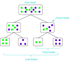
Let’s say we have 200 apples and oranges mixed together. Out of the 200, 60 are oranges. As majority is apple, if we classify everything as apple, then we have got 60 wrong. Thus in the very first node (root node) of the tree, we can say we have 60 misclassification. Next, we could split them further based on their weight into 2 splits and may be based on color into further 2 nodes each. Thus based on weight and color, we have got 4 nodes as shown below,

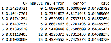
Let’s say, we still got 15 misclassification at this stage with 4 nodes. The relative decrease in error by adding 3 nodes (from 1 root node to 4 leaf nodes-> 3 nodes added) is (60-15)/60=45/60=0.75. Thus decrease per node is 0.75/3=0.25. Thus, the alpha value of this split is 0.25. We can set a limit for alpha such as 0.015 (for example). We can grow a full tree using in-sample data and cut the tree where the relative decrease in error per node for any branch (or new section) goes below 0.015.

While we can build the model using training data and test the performance with test data, there is also another method to do it – which is called cross-validation. In cross-validation, data are split into n non-overlapping groups and runs n experiments. In each experiment, n-1 groups are used to train a model and the model is tested on the left out group. The results are summarized over the n experiments. This gives a mechanism to test a model repeatedly on data that was not used to build the model. The ‘xerror’ from the above table gives us cross-validation error value.
For decision trees, it is a common approach to choose the tree with minimum cross validation error. Thus, for above sample case, we could stop the split at n=5 as it has minimum xerror value.
Conclusion:
In this blog, we discussed about how to decide the pruning point for decision tree using relative error decrease and also about cross-validation and how to use ‘xerror’ to decide on number of splits.

