Decision trees are very powerful and vey flexible machine learning techniques that allows us to do both classification and regression. In this blog, I would explain the underlying principles on which decision trees are built. In following blogs, I would also explain how decision trees tend to overfit the data, and how we could trim the decision tree – which is called as ‘Pruning’.
There are different kinds of decision trees and here the focus is on CART- Classification And Regression Trees. In classification problems, our target is a categorical variable. We are trying to understand how a set of independent variables end up dictating which category a particular observation belongs to. And, in regression problems, again we are interested in understanding how a set of independent variables are dictating the value of our dependent variable but here the target/dependent variable is a continuous variable which could be any real number. Some examples for classification problems are identifying spam or not, deciding whether to admit to ICU or not, whether to lend money or not, and any case where you want to classify observations into different categories. On the other hand, some examples for regression problems are predicting stock returns, predicting weather data, pricing a house or predicting sports score-all of those that have output in continuous range.
First, I would explain about classification problem and all the concepts hold true for regression as well. The only difference is, in classification, the output is a category whereas in regression the final value that a leaf holds is a real number.

Classification
In classification, the idea is to visualize the data points and group them into different territories based on the distribution of different classes. It is easy to visualize in two-dimensional space, however in most real-world problems, we handle cases with more than two independent variables. Thus, we might need to visualize in multi-dimensional space which is not easy to do manually.
The intention is to divide the observations into groups where similar items are clubbed. When all the observations in a group are alike, we call it a pure group. We need a measure of impurity in-order to go further in our classification. Different algorithms use different metrics to measure the best grouping. These metrics measure how similar a region or a node or a group is. Larger the impurity metric value- larger the dissimilarity of the nodes/regions data. Some examples for impurity metrics are Gini impurity, Entropy and Variance.
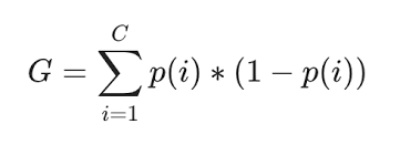
Here, I will explain about Gini impurity as it is commonly used in CART algorithms. Gini impurity is a measure of how often a randomly chosen element from the set would be incorrectly labeled if it was randomly labeled according to the distribution of labels in the subset. It can be computed by summing the probability of an item with label i being chosen (pi), times the probability of a mistake (1-pi) in categorizing the item. Simplifying it, below is the formula for Gini impurity,

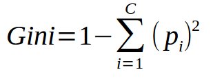
As sum of all (pi) is 1, it could be simplified as shown below,

Say, you have two items – apples and oranges mixed randomly. In a particular region, if there are all apples, then probability of finding apples(pi) is 1 and probability of a mistake (1-pi) is 0. Thus product of both is 0. Also, probability of finding an orange in this region (pi) is 0 and probability of a mistake (1-pi) is 1, which makes their product to be 0. Thus, Gini impurity is sum of 0s in this example and the group is called a pure group.
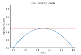
If the region is a mix of 50% apples and 50% of oranges, then it becomes the most impure group and its Gini value would be 0.5.
As shown in below graph, the groups with Gini value around 0.5 are the most impure groups.

Conclusion
In this blog, I have given introduction to decision trees algorithms, deep dived into CART and explained Gini impurity metric. In my next blog, I would explain how decision trees tend to overfit the data, and how we could do pruning using some examples.
