In this blog, I will discuss about the basics of the most popular data-science and supervised learning technique which is linear regression.
Linear regression tries to establish linear relationship between two or more variables. Let’s start with some simple two variables examples:
- people’s height and weight
- product price and sales
- advertising budget and sales
- no. of study hours and marks
- weight of car and its mileage
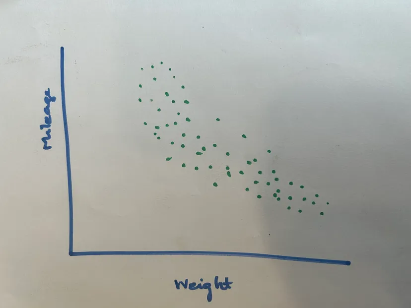
Diving deep into one specific example- “Does heavier car have lower mileage?”
Intuitively, the initial answer might be ‘Yes’. But let’s look at the data and check if we see any pattern or relationship between these two variables. Most likely the plot between these two variables would look something like this shown below,

From the pic, we can see a rough negative trend so we can simply answer to the questions by saying ‘yes, heavier cars have lower mileage on an average’.
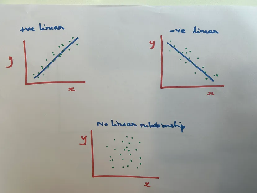
Here, when we are talking about relationship between variables, we would be looking only at linear relationships (where we can draw a straight line as shown in below picture). When we plot two variables and do not see any straight line fitting those points, then there is no linear relationship.

Now, we know what the nature of relationship between two variables is, but we do not yet know about the strength of the relationship. It is very difficult to find the strength using visual representation and it could be misleading as well.
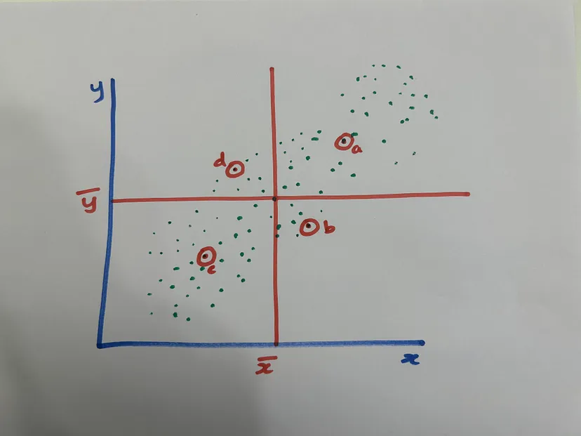
We need a specific way to quantify this relationship. The most common way of linear association is correlation or Pearson’s correlation. Let’s try to understand this concept with the help of below picture.


Any point that lies in the first or third quadrant contributes to the positive association between the two variables. Similarly, any point that lies in the second or fourth quadrant contributes to the negative association between the variables. We need a way to find the net association from all positive and negative points.

While for data points in 2nd and 4th quadrant, the values will be negative. When we take the average of this value from all the data points, we get net association strength of the two variables. This is called covariance between two variables,

Larger the covariance value, greater is the positive association between the variables, while lower the covariance value, greater is the negative association. If the value is around zero, that means that there is no linear relationship between these two variables.
Variance of a variable is nothing but covariance with itself,

Covariance is a very good measure of association, but it has its problems. It is sensitive to its units. The unit of covariance is the product of units of x and y. If we change unit of 1 variable for example, unit of x from centimeter to kilometer, then the covariance value changes. So, simply looking at covariance, we can never say if the association is strong or weak as it really depends on the units.
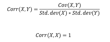
Let’s standardize it by getting rid of its units. That’s what we call as correlation. Correlation is Covariance divided by (std. deviation of x and std. deviation of y).

The correlation of a variable with itself is 1 and that’s the max correlation possible.

And correlation of a variable with its negative-self is the -1 and that’s the min correlation possible.
Thus, the correlation is always within the range of (-1 to 1) which makes it easy to interpret its value. If the correlation between two variables is 0.9 then that means, there is strong positive association between those two variables; any negative value would mean negative association and any value around 0 would mean no association.
The important point to note here is correlation is not causation. Let’s see this with an example. Let’s say for our former example of cars- the correlation between the weight of the car and mileage is -0.85, which is a strong negative association. So, we can conclude that heavier cars tend to have lower mileage. But, we cannot conclude that decreasing the weight of the car increases the mileage or vice versa. There could be several factors affecting the mileage, so the correlation between weight and mileage doesn’t mean causation.
In this blog, we started with visual representation of linear relationship for two variables and explored fundamental topics such as covariance and correlation. These concepts help us build strong foundation for understanding linear regression (bivariate and multivariate) techniques. Hope you found this helpful 🙂
Happy learning & relearning!!
Also published on medium.com
