Classification is a supervised algorithm where we are trying to predict the dependent variable. In classification, it is either or category. Eg: Pass/Fail or Yes/No. Whether student pass or fail is classification problem whereas what score the student secures is a linear regression problem.
For example, “How likely a student is to complete a course if the student studies for 50 hours?” is a classification problem.
We could have multiple independent variables and we could have multiple categories for dependent variable.
In our example, when we plot no. of study hours and Yes/No status, we see data points in two levels as shown in below picture,

If we try to fit a straight line, we get an equation for these data points which can be used to find a probability of completing or not. As a rough method, we could consider everyone above 0.5 score as Yes and everyone below 0.5 probability-score as No. This method not just predicts whether a student would complete or not, but tells the probability to complete or not-complete. Some people still use this method. However, this method has various problems with it and it can easily be much better.
The first problem is the data doesn’t fit in the straight line. The straight line can extend beyond 1 or go below 0- which doesn’t make sense for a probability score as we expect the probability score to be between 0 and 1. The second problem is that the marginal rate is constant for a straight line fit, whereas the change in probability score is not actually constant for different marginal rate. Finally, with the straight line fit, we are never ever right as none of the data points actually lie on the straight line. We want the model such that it covers most of the data points and straight line doesn’t goes thru the data points.
So instead of force fit a straight line, we want to find a model that flows through and explains as much data as possible.

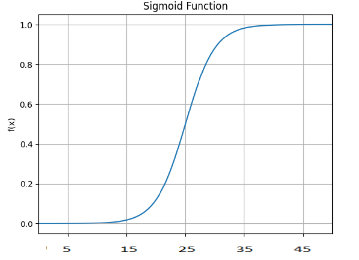
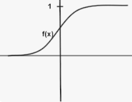
Maybe we need a model that interpolates between the two categories. This is a better fit for the data. Curves of this kind that looks like a S are called Sigmoid curve. These sigmoid curves do an extremely good job in classification problems. They start out at 0 and flat out at 1. Zero could be one category- ‘No’, and One could be another category- ‘Yes’. Sigmoid curves have this real ability to be minimal at 0 and maximal at 1, flatten out at those two extremes and be able to provide smooth interpolation between.
Y= a+bx is for straight line
For sigmoid, it would be Y=f(a+bx) where f would be some kind of sigmoid function.
The two most popular choices for f() are:
- Logistic regression- Logit function
- Probit regression- Probit function (cumulative distribution for normal distribution)
We are going to focus only on logit function as that is the most common sigmoid function used in classification problems.
What logistic regression does is to find the best fit logit function for the given data. Though it is called regression, it is a classification problem and the reason we call it regression is because it follows the process of fitting a line/curve to the data.
Of all the logit functions that are possible with the different a and b in the equation,

X could be between -infinity to +infinity and thus denominator could be between 1 and infinity and the entire equation could be between 1 and 0.
Thus, y is always between 0 and 1.
Log of odds ratio is linear and can be written as shown below,


That’s how the logit function has an easy and convenient explanation as it is same as log of odds ratio.
Now, coming back to finding the best a and b for the model fit,
In linear regression, we minimized sum of squared residuals. This unfortunately will not work in logistic regression. As the logit function has a function that’s more complex than simple linear equation, the square of the function becomes very complex and when we try to minimize the square, there might be more than one solution.
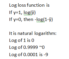
So, instead of sum of residual-square, we try to minimize the log loss or cross-entropy.

So, for correct predictions, log(ŷ) will be close to 0, while for wrong predictions, it will be higher value.
Similarly, for when y=0, -log(1-ŷ) will be close to 0 for correct predictions and close to 9 for wrong predictions.
The log loss function is written as

Correct classifications reduce to minimize the log function whereas wrong classifications increase the log loss value. If we find a curve that minimizes the log loss value, then that’s the curve with least number of misclassifications.
When we have more than one independent variable, then logistic regression model tries to fit a S-shaped curved surface on the multi-dimensional space.
The logit function becomes,

Lastly, the pros and cons of logistic regression
Advantages:
- The classification model that gives probabilities
- Quick to train and predict for unknown records.
- Can easily to extended to multiple classes.
Disadvantages:
- Assumes that variables are independent. No interaction terms.
- Interpretation of coefficients is difficult.
Depending on the cost of misclassification, we can decide the threshold for different classes in the dependent variable.
For each different threshold we decide, we could have different confusion matrix.
It is matrix between truth and predictions- dividing your predictions into True Positives, True Negatives (correct classifications), False Positives and False Negatives (misclassifications).
More about the metrics used in logistic regression in the next article…
Happy learning!!
Also published on medium.com
